
 KonfAI
KonfAI on real data#
See KonfAI do the work on real medical-imaging data: a regional read from a
1.06-billion-voxel OME-Zarr pyramid, nine deterministic transforms, six sampled
augmentations, and a complete deformable registration. The transform and
augmentation panels use one axial CT slice from a real paired abdominal case
(1ABB124, SynthRAD 2025 Task 1, CC BY-NC 4.0). Every processed panel is
generated by the actual KonfAI class or App named in its title; no patient
identifier or image metadata is retained in the PNG. Dataset attribution and
hashes are recorded in the
visual asset provenance manifest.
The images are explanatory, not a recommendation for clinical preprocessing. Choose ranges and probabilities from the intensity distribution, voxel spacing, anatomy, acquisition protocol, and invariances of your task.
Scale: a real OME-Zarr regional read#
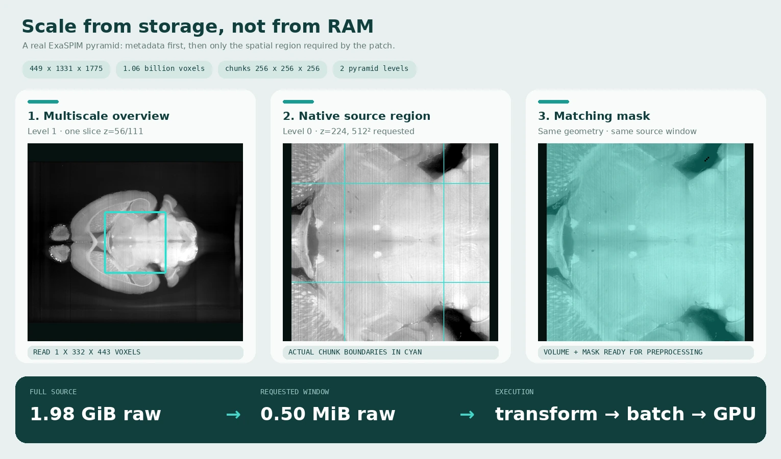
The source is a real two-level ExaSPIM OME-Zarr store from AIND specimen
822175 (CC BY 4.0). KonfAI reads its metadata, one coarse plane, one 512²
native window, and the matching mask window. The figure therefore visualises
the storage-to-patch path itself rather than an artist’s diagram. See
Processing large images for the execution rules and exact reproduction
command; the provenance manifest
records the public source and hashes.
Deterministic transforms#
Transforms run in training, prediction, and evaluation wherever they are declared. Their state can also carry the information required to invert an operation when predictions are written.
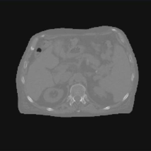
SourceReal paired abdominal CT · unchanged HUMIN −1024.00 · MEAN −586.57 · MAX 979.32 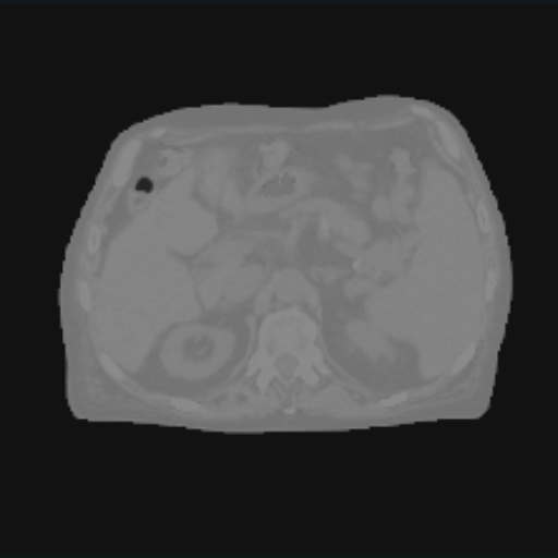
ClipValues above 100 HU flattened · same display windowMIN −1000.00 · MEAN −575.52 · MAX 100.00 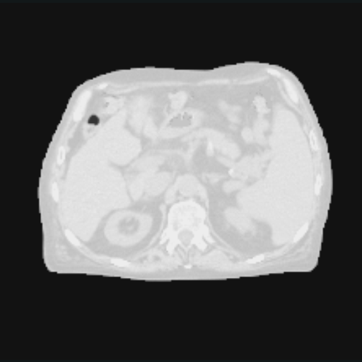
NormalizeTarget numerical range [−1, 1]MIN −1.00 · MEAN −0.23 · MAX 1.00 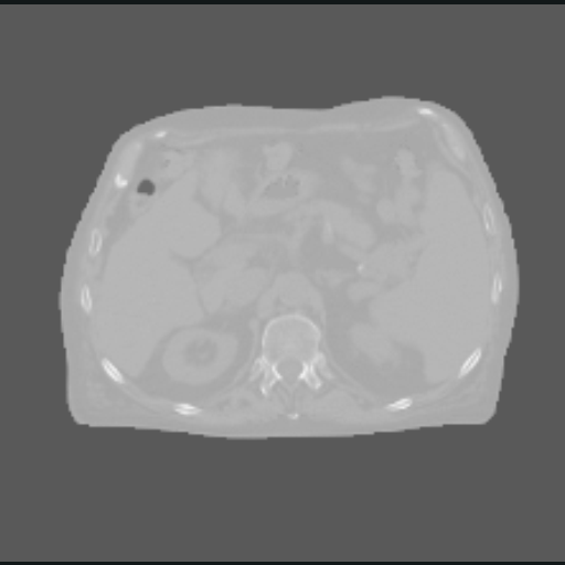
StandardizeAutomatic mean and standard deviationMIN −0.87 · MEAN 0.00 · MAX 3.11 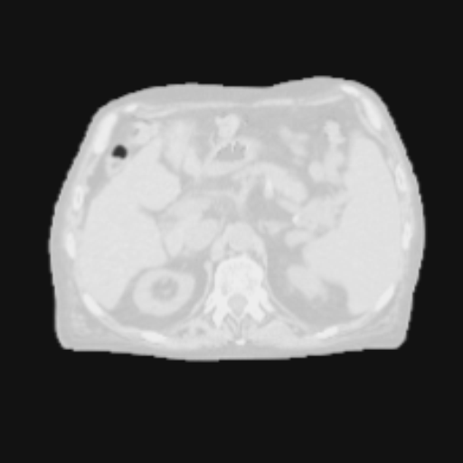
Resample to shape219 × 222 → 220 × 220 voxelsOUTPUT GRID 220 × 220 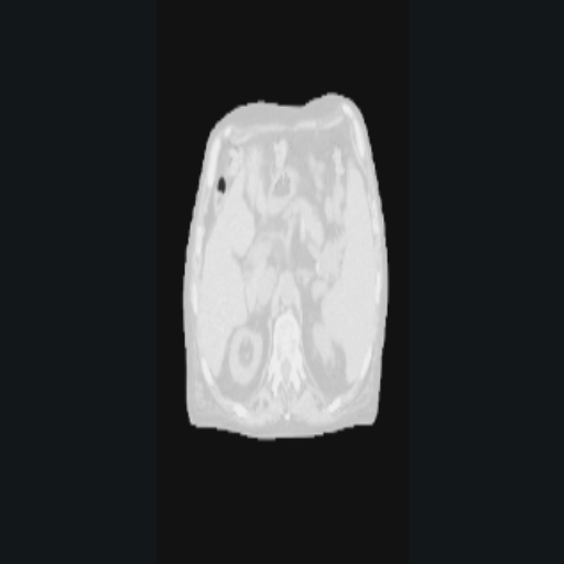
Resample spacing0.80 × 0.80 → 1.25 × 0.55 mmGEOMETRY-AWARE INTERPOLATION 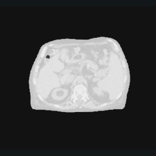
PaddingConstant −1 border around the source grid[28, 28, 18, 18] VOXELS 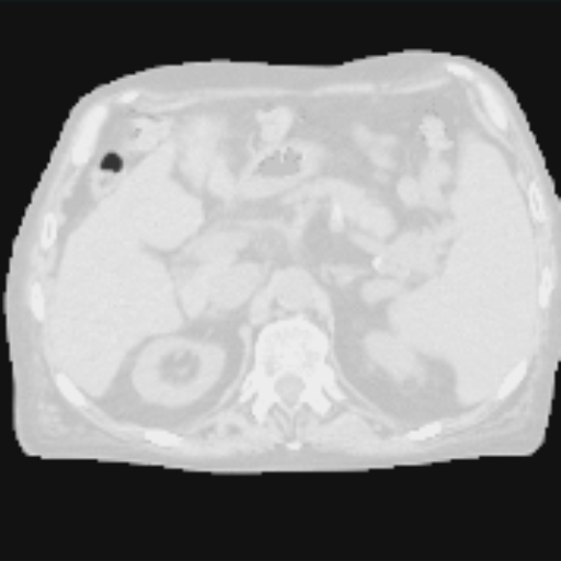
CropConfigured central ROI with geometry updateROI 177 × 178 VOXELS 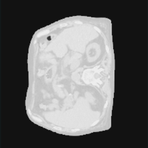
Permute axesSwap the two spatial dimensions219 × 222 → 222 × 219 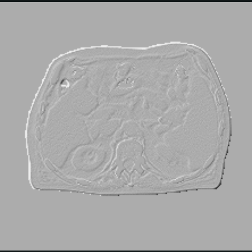
GradientSpatial edge magnitudeMIN 0.01 · MEAN 0.71 · MAX 1.40
One source slice, nine direct KonfAI transform outputs.Open any card independently · real abdominal CT · intensity, grid, spacing, orientation, and edge operations
Matching YAML:
groups_dest:
  CT:
    transforms:
      Clip:
        min_value: -1000
        max_value: 100
      Normalize:
        min_value: -1
        max_value: 1
        inverse: true
      ResampleToResolution:
        spacing: [1.25, 0.55]
        inverse: true
      Padding:
        padding: [28, 28, 18, 18]
        mode: constant:-1
Clip flattens values above 100 HU so the bright cortical bone disappears; its
panel deliberately keeps exactly the same [-1000, 1000] HU display window as
the source. Every card uses the same classic medical grayscale, with only the
pure black and clipped white endpoints softened; tensor values are unchanged.
Normalize preserves the relative anatomy
while changing the numerical range. Standardize centers the distribution and
scales it by its standard deviation; its visual appearance depends on the
display window, which is why each card also reports min, mean, and max. The
spatial cards make geometry changes explicit: resampling reports
the source and destination shape or spacing, padding expands the grid, crop
updates the region of interest, Permute swaps axes, and Gradient exposes
spatial edges. Every panel is the direct output of the named KonfAI class.
Random augmentations#
Augmentations are sampled per case and shared by every patch of that case during an epoch. The fixed seeds used to build this page make the documentation reproducible; normal training draws new states after the epoch reset.
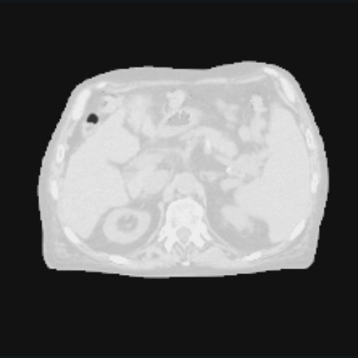
SourceShared clipped and normalized referenceFIXED DOCUMENTATION SEEDS 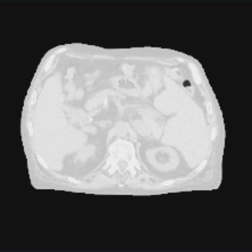
FlipDeterministic horizontal samplef_prob [0, 1] 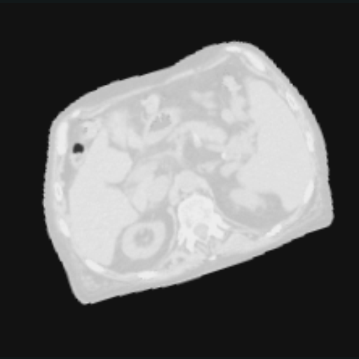
RotateSpatial transform shared across the casea_min 18° · a_max 18° 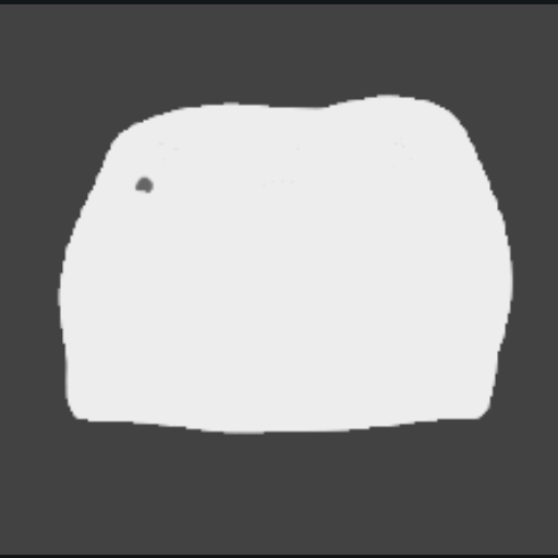
BrightnessSampled intensity offsetb_std 0.35 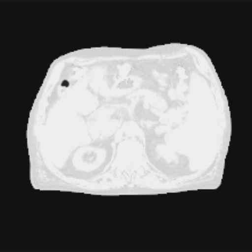
ContrastSampled intensity scalec_std 0.75 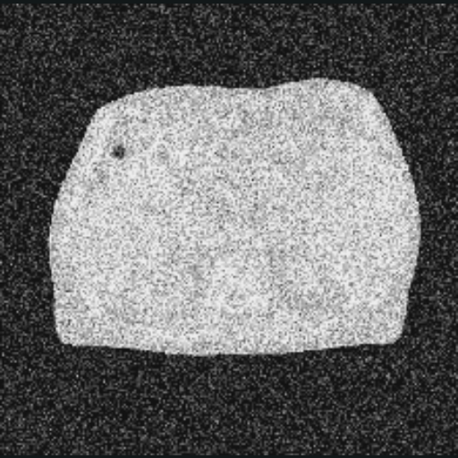
NoiseSampled below a 55% timestep ceilingn_std 0.65 · prob 0.55 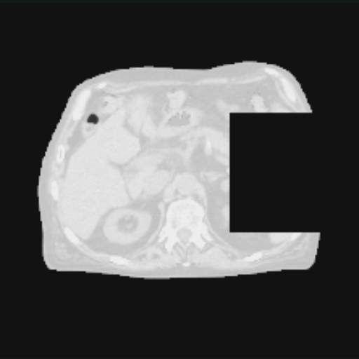
CutOUTRectangular region replaced by −1cutout_size 0.34 · c_prob 1
One source image, six sampled augmentation states.Open any card independently · fixed documentation seeds · shared spatial state across a case
One typical training block (the fixed documentation render forces each shown state to run so the visual comparison is deterministic):
Dataset:
  augmentations:
    SpatialAndIntensity:
      nb: 1
      data_augmentations:
        Rotate:
          a_min: -18
          a_max: 18
          prob: 0.5
        Contrast:
          c_std: 0.75
          prob: 0.3
        Noise:
          n_std: 0.65
          prob: 0.55
Important
For Noise, prob controls the maximum diffusion timestep rather than a
standard apply/do-not-apply probability. For spatial transforms, label maps
follow the same sampled geometry and use nearest-neighbour interpolation.
Registration: moving image to physical field#
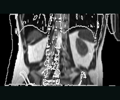
01 · INPUTMoving MR — beforeFixed-CT contours expose the controlled offsetNCC 0.129 · MAE 106.11 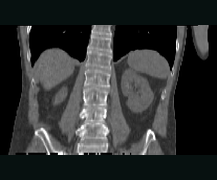
02 · REFERENCEFixed CT targetReference geometry and output grid222 × 226 × 124 · 2 MM GRID 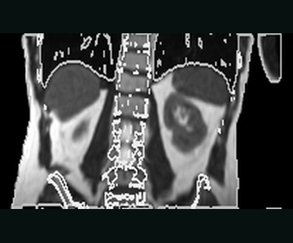
03 · OUTPUTMoved MR — afterConvexAdam_Composite output on the fixed gridNCC 0.937 · MAE 21.09 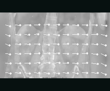
04 · FIELDDisplacement fieldThree physical components with sampled vectorsMEAN 23.06 MM · P95 25.55 MM
One real moving/fixed pair, one executed IMPACT-Reg App.Open each stage independently · ConvexAdam_Composite · NCC 0.129 → 0.937 · moved image + DVF + reusable transform
The input is de-identified SynthRAD 2025 Task 1 abdomen case 1ABB123
(CC BY-NC 4.0), with a controlled metadata-only offset. Full attribution and
hashes are in the
asset provenance manifest.
The App writes the moved MR, a three-component displacement field in
millimetres, and a reusable transform on the fixed CT grid. The documentation
generator reads and validates every plane from the real moving and output
volumes; it does not reconstruct a decorative before/after image. See
Using KonfAI Apps for the exact preset, measurements, evaluation, and Slicer
workflow.
How the figures stay trustworthy#
Recreate the same transform sequence on the maintained public quickstart case:
hf download VBoussot/konfai-demo Segmentation/1PC006/CT.mha \
  --repo-type dataset --local-dir /tmp/konfai-doc-gallery
pixi run --environment dev python docs/scripts/generate_visual_gallery.py \
  --input /tmp/konfai-doc-gallery/Segmentation/1PC006/CT.mha \
  --slice-index 49
The public command deliberately substitutes a different case, so it validates the transform logic rather than reproducing the committed pixel values. The dimensions and numerical captions above describe the committed 1ABB124 slice; update them if you replace those assets with another case.
The generator imports Clip, Normalize, Standardize, both resampling
variants, Padding, Crop, Permute, Gradient, and every named augmentation
directly from KonfAI. It drives augmentations through their public per-case
lifecycle. The committed board uses the real abdominal CT case 1ABB124;
the command above offers a maintained public alternative with different anatomy
and identical transform logic. Both paths extract only the selected axial
plane. If --input is omitted during local experimentation, the script falls
back to a procedural phantom; that fallback is never used to represent an App
prediction. The registration board is built separately by
generate_registration_proof_gallery.py from completed App outputs and
validates fixed-grid geometry plus decoded moving/reference voxel equality one
plane at a time.
Next steps#
Transforms — every transform and argument
Augmentations — every augmentation and lifecycle detail
Segmentation Example — use preprocessing and augmentation in a complete task
Using KonfAI Apps — reproduce registration, evaluation, uncertainty, and Slicer delivery