
 KonfAI
Processing large images#
Use this guide when a case is too large to materialise comfortably in RAM, or when you want OME-Zarr, HDF5, DICOM, or ITK storage to participate directly in patch loading. KonfAI can request regional windows from these backends, but whether a workflow actually streams is determined by both the dataset settings and the transform chain.
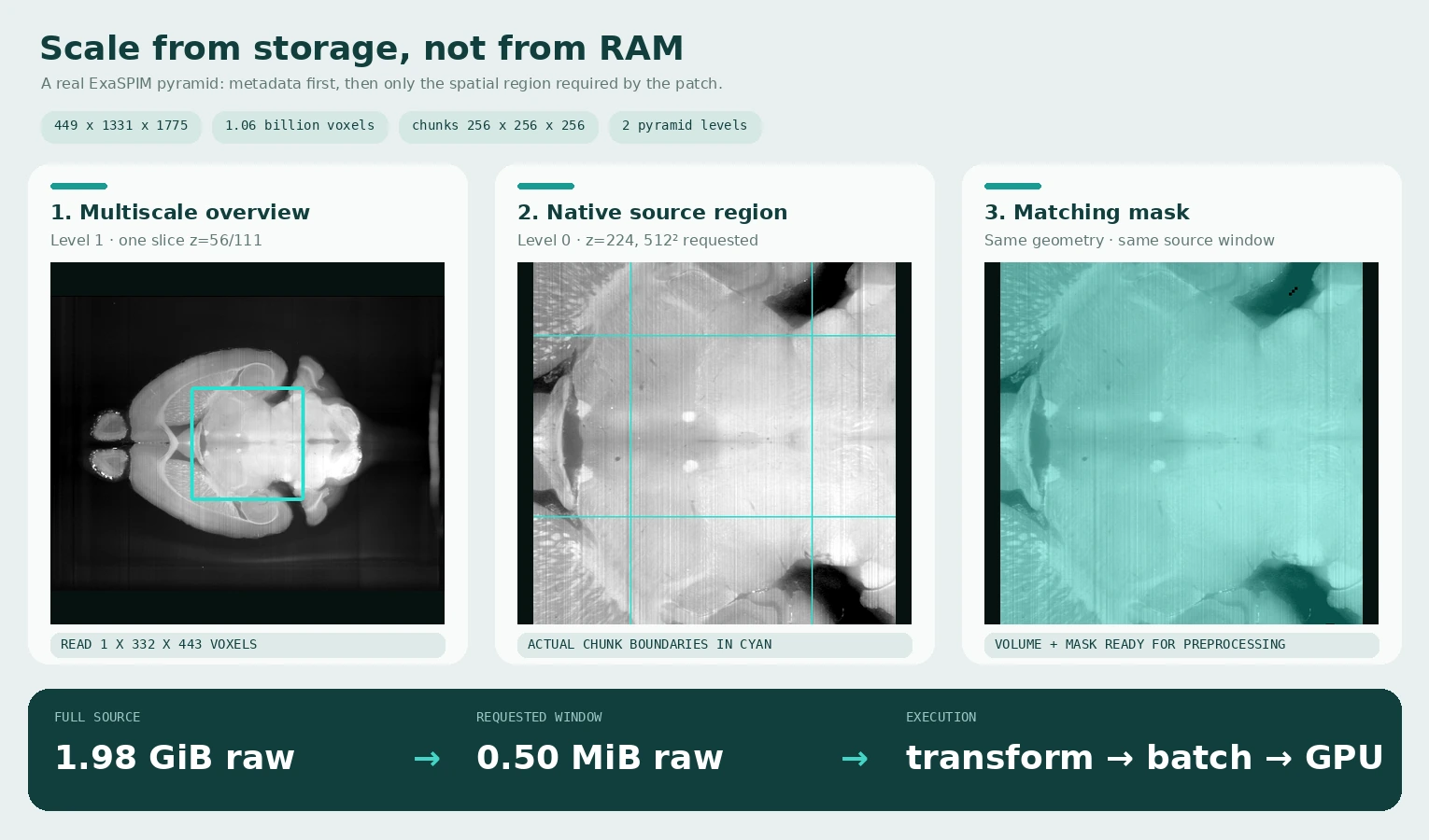
This is a real regional read from AIND ExaSPIM specimen 822175 (CC BY 4.0),
not a synthetic volume. The public source and derivative hashes are recorded in
the visual asset provenance manifest.
Level 0 contains 449 × 1331 × 1775 uint16
voxels (1.98 GiB uncompressed) in 256³ chunks. The figure reads one coarse
level-1 plane to locate the field of view, then asks KonfAI for one 512² region
at native resolution and the identical region from the mask. Only 0.50 MiB of
image pixels is materialised for that native plane window.
Choose the memory regime#
Streaming is derived from the pipeline; there is no streaming: true switch.
The workflow’s default, the optional memory_budget, and the transform chain
lead each case and augmentation draw to one of three regimes:
Regime |
When |
Memory held |
|---|---|---|
Cache |
the training default |
Every case, resident across epochs. |
Stream |
predict/eval default or budget exceeded; chain streamable |
The source region for one patch. |
Buffer |
same triggers; the chain needs a whole volume |
A FIFO of |
memory_budget drives the memory lever of each workflow: in training it
chooses cache versus stream/buffer; in evaluation it sizes the auto-patch.
Prediction and evaluation are always one-pass (stream/buffer), never cached.
A number is interpreted as GiB, strings may include units, and auto offers
80% of the detected per-rank memory limit. It is a size estimate—not a hard
allocator limit—because transformed shapes, augmented copies, and transient
construction peaks are not included. See Patch streaming for the
exact precedence and Training configuration for shuffle_window.
Dataset:
  dataset_filenames:
    - ./Dataset:omezarr
  memory_budget: auto
  batch_size: 2
  num_workers: 4
  Patch:
    patch_size: [64, 128, 128]
    overlap: 16
The equivalent source selector for a DICOM-series dataset is
./Dataset:dicom; dcm means a single file handled by SimpleITK, not the
DICOM-series backend. See Storage backends & formats for
the exact layouts and format tokens.
How the spatial planner derives a source read#
Every transform declares its patch locality: exact voxel, bounded halo, orientation remap, crop translation, global statistic, rescale, or whole volume. KonfAI walks the transform and sampled-augmentation chain and maps the requested output patch back to the source region on disk.
Locality |
Representative built-ins |
Regional work |
|---|---|---|
Pointwise |
fixed-bound |
Read the exact patch. |
Global statistic |
|
Stream the statistic once, then read the patch. |
Halo |
|
Enlarge the read and crop the result. |
Orientation |
|
Remap indices to the source. |
Crop |
|
Translate the target region. |
Rescale |
|
Map through scale and add interpolation context. |
Whole volume |
masked transforms, histogram matching, arbitrary displacement |
Use the bounded buffer. |
Region stages compose — any number of them, each pulling its read through the
one before it — so a chain of remaps/halos/rescales still streams. An undeclared
custom transform, an excessively large halo, or a global statistic after a
value-changing stage selects the safe whole-volume path. WHOLE_VOLUME is the
default for custom transforms, so missing locality metadata reduces performance
rather than silently changing results.
The backend must also serve a disk region efficiently. HDF5 and OME-Zarr do so
natively, DICOM reads selected slices, and SimpleITK supports regional reads for
uncompressed MetaImage and non-gzipped NIfTI. Compressed/unsupported formats
still return correct patches but may decode the volume for every request, with
a warning. A single-store HDF5 file is serialized per process: a streamed write
into it (a Save materialization, a prediction sink) holds the store for its
whole duration, so same-process threads reading other cases from that file wait.
The complete planner rules, built-in declarations, equivalence
tolerances, and custom-transform contract live in Patch streaming.
OME-Zarr layout and levels#
Use one store per case and group:
Dataset/
├── CASE_001/
│   └── CT.ome.zarr/
└── CASE_002/
    └── CT.ome.zarr/
The selector may include a pyramid level, for example omezarr@1. KonfAI reads
metadata through get_infos() and touches only chunks intersecting the selected
window during a regional read. Chunk shape still matters: chunks much larger
than patches increase unnecessary I/O; very small chunks increase metadata and
decompression overhead.
The figure above is reproducible when the local ExaSPIM store is available:
pixi run --environment dev python docs/scripts/generate_scale_gallery.py \
  --root /path/to/ExaSPIM_Template/Data/Dataset_prepared \
  --case 822175
The generator calls Dataset.get_infos() for metadata and
Dataset.read_data_slice() for every displayed region. It never calls
read_data() or converts the full store to an in-memory array.
Dataset patching versus model patching#
These solve different problems:
Dataset.Patchcontrols what the dataloader sends to the model. Use it to bound source, preprocessing, batch, and forward memory.Model.ModelPatchsplits data again inside a KonfAI network. Use it for a heavy subgraph, a 2D/2.5D model inside a 3D workflow, or intermediate patch-level supervision.
Do not add model patching merely because dataset patches overlap. Start with
dataset patching, then add ModelPatch only if a network stage has a separate
memory or dimensionality requirement. See Model graph and output naming.
Tune in this order#
The default
memory_budget(auto) already decides from the dataset’s size; set an explicit value below the dataset’s size to force the stream/buffer path.Leave
patch_sizeaxes at0so the framework sizes them (the whole volume when it fits, a measured shrink on OOM), or pin the largest size that fits the model and required context.Start with
batch_size: 1; increase it while measuring throughput and VRAM.Add overlap only when border quality requires it. More overlap means more reads and forward passes.
Increase
num_workersuntil storage or CPU preprocessing is saturated.Try
pin_memory: truefor CUDA transfer, then measure; it consumes locked host memory and is not universally faster.Use
prefetch_factoronly with worker processes and account for the extra prefetched batches in RAM.
Prediction may keep a reassembly accumulator on the GPU when it fits and fall back to CPU accumulation when it does not. Mean/Cosinus overlap blending and Mean/Median/Concat model or TTA reductions have different memory costs. The canonical prediction fields are in Prediction configuration.
When the reassembled output itself is the memory peak, streaming handles it
automatically — there is no flag to set. Each output slab is finalized and
written to disk as soon as its patches complete, so peak RAM is one patch window
instead of the whole volume. Geometry inverses stream too, and they compose:
a Canonical/Flip/Permute inverse remaps each slab to its written region, a
Padding inverse crops it in flight, a ResampleToResolution/ResampleToShape
inverse resamples back through a sliding window — chained in any number, each
pulling through the next — so a huge output at ORIGINAL resolution is written
slab by slab without ever being held whole. A masked finalize (Mask) streams
too: each slab reads only its aligned mask region. What streaming cannot honour
(a whole-volume transform or a destination without region writes) splits
instead: the pointwise prefix still streams into a light post-reduction buffer
and the remaining stages run once on it. Only a TTA draw whose inverse moves the
slab axis (a z-flip, a z-moving permute), a TTA case too light to be worth the
slab-synchronized reduce, or a non-voxel-local reduction keep the whole-volume
path. A streamed case is voxel-identical to the assembled path on a
given device, except a linear-resample inverse, which streams by default and
matches the whole-volume F.interpolate to float rounding rather than
bit-for-bit. KONFAI_STREAMED_WRITES=0 forces the whole-volume path globally.
A float (linear) resample inverse — resampling probabilities/logits back to
the native grid before an argmax — streams within the sliding window by
default like the other geometry inverses. On a large multi-class output the
whole-volume F.interpolate is otherwise the memory peak (tens of GB), and a
combine: Concat ensemble makes it worse by keeping every member’s channels in
the tensor being resampled; streaming bounds both. It matches the whole-volume
F.interpolate to float rounding, not bit-for-bit — argmax’d labels absorb it
(a boundary voxel or two may flip; a raw float output differs by ~float-rounding).
Set KONFAI_STREAM_LINEAR_RESAMPLE=0 to force the exact whole-volume linear
resample when you need bit-identity or the per-member stack; resampling the
argmax’d labels (a nearest, streaming resample) or collapsing members with
combine: Mean/Median first also avoids the peak.
Verify the behaviour you care about#
Do not infer streaming from a successful run alone—the fallback is designed to remain correct. Measure peak RSS and storage reads on a representative case, and compare the same model, patch size, overlap, TTA, batch size, workers, and hardware when evaluating performance.
KonfAI currently has no committed framework-wide benchmark against MONAI or nnU-Net under those controlled conditions. The regional-read mechanism is implemented and tested; general speedup claims require separate evidence.
Common failures#
RSS still scales with case size: the planner selected the bounded whole-volume path for that case or augmentation draw. Inspect the locality rules, or preprocess the unsupported operation once with
Saveand stream from that materialised dataset. TheSaveitself streams: when the transforms before it stream, its cache is written slab by slab on first access — the volume is never assembled, even the first time.OME-Zarr is slow: inspect chunk shape, compression, pyramid level, worker count, and overlap. Avoid assuming more workers always improve remote storage.
Output seams are visible: add overlap and select a compatible
patch_combine; confirm patch read and reassembly ordering has not been changed by custom code.CUDA OOM occurs after forwards complete: the volume-sized output or reduction may be the peak. Reduce output channels/TTA/ensemble size or let the predictor use CPU accumulation.
Next steps#
Storage backends & formats — backend capabilities and exact layouts
Patch streaming — planner rules, locality table, and fallbacks
Training configuration — loader, cache, patch, and worker fields
Prediction configuration — batching, TTA, ensembles, reduction, and output writing